
Investing Wisely: An Explainable AI Approach to Identifying Profitable Companies
6 June, 2024
The application of advanced machine learning (ML) methods has revolutionized investments in public companies, offering high computational power and accuracy. However, the opaque nature of these models poses a significant challenge for informed decision-making. This article delves into an innovative explainable AI (XAI) model designed to analyze corporate financials and predict expected returns by assessing credit risk and profitability. Utilizing Shapley values, this model interprets AI-generated predictions, enhancing transparency and trust. Empirical analysis of 1,700 public companies' financial performance demonstrates that expected returns can be reliably forecasted and elucidated by a combination of financial indicators, thus aiding investors in making well-informed decisions.
Introduction
Artificial intelligence (AI) has emerged as a transformative force across numerous domains, with finance being a prominent beneficiary. From algorithmic trading to risk management, AI's potential to process vast amounts of data and generate actionable insights is unmatched. However, the inherent complexity and "black-box" nature of many AI models pose significant challenges. Investors and financial analysts often find it difficult to trust models they cannot interpret. This dilemma has given rise to explainable AI (XAI), which strives to balance the high accuracy of complex models with the need for transparency and interpretability.
Complex ML models have demonstrated exceptional performance in tasks such as credit scoring, portfolio optimization, and profit prediction. Yet, their lack of interpretability limits their utility in finance, where understanding the rationale behind decisions is crucial. To address this, model-agnostic methods like Shapley values have been developed. These methods offer a way to explain the predictions of any machine learning model, regardless of its complexity, by attributing the output to the input features in a manner akin to cooperative game theory.
In this article, we focus on investment decisions in public companies trading on NYSE, AMEX and NASDAQ. By leveraging a machine learning model to predict Company's expected returns with high accuracy, we propose an explainable AI framework that uses Shapley values for interpretability. Our methodology follows a five-step process: estimating the probability of default (PD) using the XGBoost algorithm, identifying significant risk factors, selecting non-default companies, estimating their profitability, and interpreting the results using Shapley values.
Methodology
Estimating Credit Risk
Credit risk estimation is pivotal in finance, as it assesses the likelihood that a company will default on its financial obligations. Traditional methods like logistic regression, while transparent, often fall short in accuracy when compared to complex ML models. Logistic regression models the probability of default (PD) as a logistic function of the input features, which can be expressed as:
PD = 1 / (1 + e-(β0 + β1X1 + β2X2 + ... + βnXn))
Here, β represents the coefficients of the model, and X represents the input features. Despite its interpretability, logistic regression is limited by its linear nature.
In contrast, the Extreme Gradient Boosting (XGBoost) algorithm, a powerful ML model, constructs an ensemble of decision trees to enhance predictive performance. Each tree in the ensemble corrects errors made by its predecessors, optimizing the model iteratively. XGBoost's objective function combines a loss function, which measures the model's predictive accuracy, with a regularization term that penalizes model complexity, thus preventing overfitting. The general form of the objective function is:
Obj = Σi=1n L(yi, ŷi) + Σj=1T Ω(fj)
where L is the loss function, Ω is the regularization term, yi are the true labels, ŷi are the predicted labels, and fj represents the individual trees.
Although XGBoost excels in accuracy, its complexity renders it a "black-box." To address this, we utilize Shapley values, which explain the output of any machine learning model by distributing the prediction among the input features based on their marginal contributions. This method, grounded in cooperative game theory, ensures that each feature's contribution to the prediction is fairly evaluated.
Estimating the Expected Return
Investment strategies aim to balance risk minimization and return maximization. For businesses, estimating expected returns is crucial as it provides insights into their future resilience and sustainability. We calculate expected returns by combining credit risk assessments with profitability measures. The formula used is:
ERi = (1 - PDi) × Pi
where ERi is the expected return for the ith enterprise, PDi is the probability of default, and Pi represents profit after tax.
This approach integrates the likelihood of default with potential profitability, offering a comprehensive view of the investment potential. Profitability is often measured through financial metrics such as EBITDA (Earnings Before Interest, Taxes, Depreciation, and Amortization), which provides a clear picture of operational efficiency, and net income on total assets, which indicates overall profitability relative to asset base.
Model Comparison
To evaluate and compare the models used for credit risk estimation, we employ binary classification metrics, specifically the area under the receiver operating characteristic (ROC) curve (AUC). The ROC curve illustrates the trade-off between the true positive rate (TPR) and the false positive rate (FPR):
 TPR = TP / (TP + FN)
FPR = FP / (FP + TN)
An AUC value closer to 1 indicates excellent model performance. For expected return estimation, we utilize regression models and assess their performance using the mean squared error (MSE), which measures the average squared difference between predicted and actual values:
MSE = (1 / n) Σi=1n (ŷi - yi)2
Model Code
Using the Python code, we follow a structured approach to predict the financial health of public companies and interpret the results using explainable AI techniques.

The first step in the code involves data preprocessing and balancing. Data preprocessing includes tasks like handling missing values, encoding categorical variables, and normalizing numerical features. The Synthetic Minority Over-sampling Technique (SMOTE) is employed to generate synthetic samples for the minority class, thus balancing the dataset and improving the model's performance.
Next, we train an XGBoost model, a highly efficient and flexible machine learning algorithm, to estimate the probability of default for each Company. XGBoost is chosen due to its high accuracy and robustness. The model is trained on various financial indicators, and hyperparameters are tuned to optimize its performance. The output is the probability of each firm defaulting on its financial obligations.
Despite the high accuracy of the XGBoost model, its "black-box" nature makes it difficult to interpret. To address this, the code calculates Shapley values, which are a model-agnostic method to explain the output of the machine learning model. Shapley values provide insights into how each feature contributes to the prediction, thus improving transparency and enabling better decision-making.
Using the estimated probability of default, we then calculate the expected return for each firm. This is done by combining the probability of default with a predictive measure of profitability, such as profit after tax. The formula used is Expected Return=(1−Probability of Default)×Profit After Tax\text{Expected Return} = (1 - \text{Probability of Default}) \times \text{Profit After Tax}Expected Return=(1−Probability of Default)×Profit After Tax. This step provides a quantitative measure of the potential return on investment for each company.
Results
Our empirical analysis involved 1,700 Companies in 2019, with their statuses (default or non-default) assessed one year later. We identified significant feature variables through F-test statistics and addressed multicollinearity using the Variance Inflation Factor (VIF). The selected features included Current Assets, Revenue, EBITDA, Debt to Equity, Total Assets, Debt, and Net Income on Total Assets.
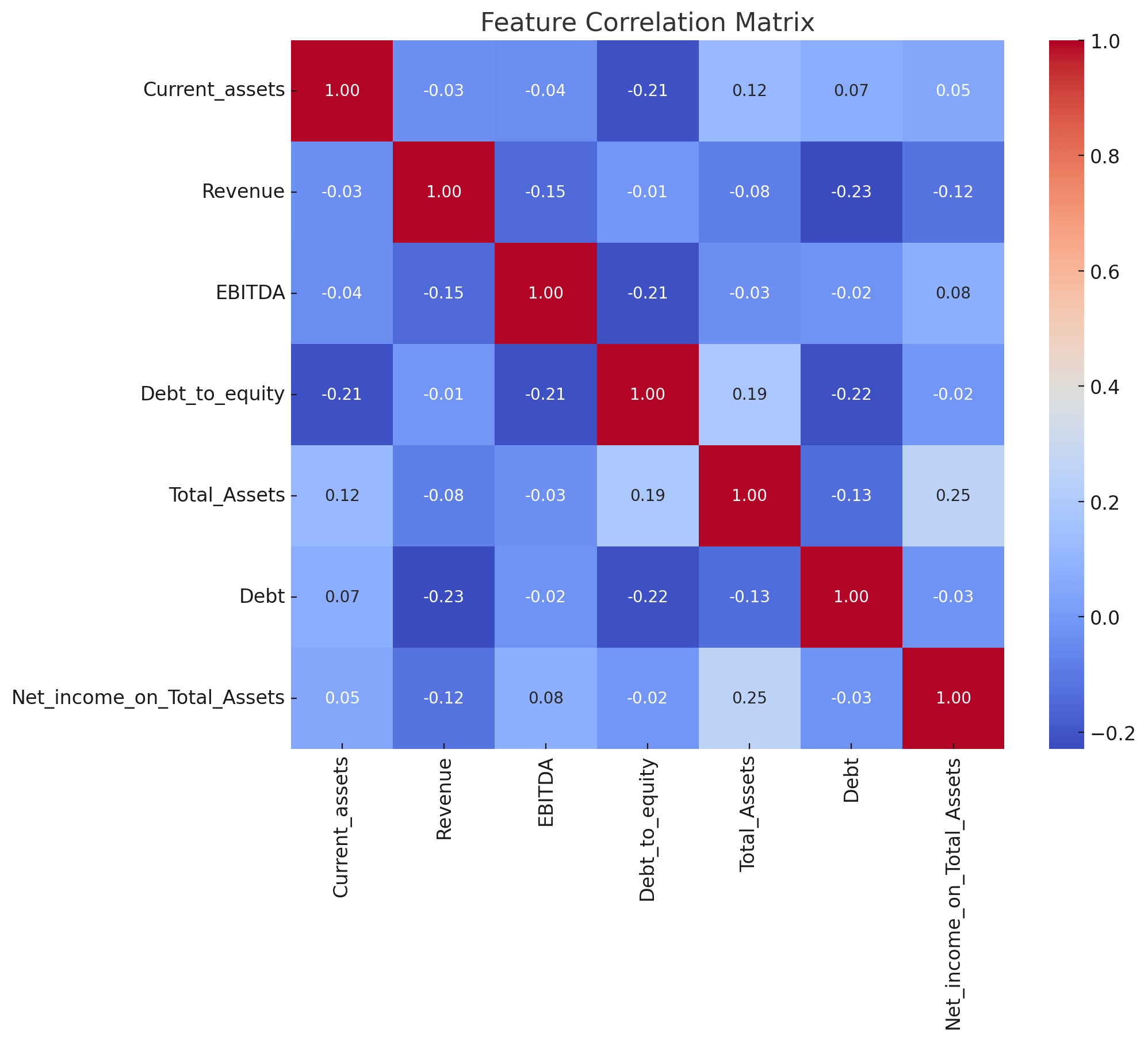
The table above represents the correlation matrix for various financial indicators of companies, including Current_assets, Revenue, EBITDA, Debt_to_equity, Total_Assets, Debt, and Net_income_on_Total_Assets. Each cell in the table displays the correlation coefficient between the row's variable and the column's variable.
The correlation matrix helps in understanding the relationships between different financial indicators. For instance, companies with higher total assets tend to have higher net income on total assets. Conversely, companies with higher revenue tend to have lower debt levels, indicating a potential inverse relationship between revenue generation and reliance on debt. This information is useful for financial analysis and investment decision-making.
| Current_assets | Revenue | EBITDA | Debt_to_equity | Total_Assets | Debt | Net_income_on_Total_Assets | |
|---|---|---|---|---|---|---|---|
| Current_assets | 1.000000 | -0.034033 | -0.037654 | -0.211882 | 0.120075 | 0.069321 | 0.047966 |
| Revenue | -0.034033 | 1.000000 | -0.146354 | -0.011783 | -0.082393 | -0.228878 | -0.115660 |
| EBITDA | -0.037654 | -0.146354 | 1.000000 | -0.214816 | -0.034695 | -0.021957 | 0.081690 |
| Debt_to_equity | -0.211882 | -0.011783 | -0.214816 | 1.000000 | 0.187530 | -0.218485 | -0.016005 |
| Total_Assets | 0.120075 | -0.082393 | -0.034695 | 0.187530 | 1.000000 | -0.133339 | 0.249953 |
| Debt | 0.069321 | -0.228878 | -0.021957 | -0.218485 | -0.133339 | 1.000000 | -0.026299 |
| Net_income_on_Total_Assets | 0.047966 | -0.115660 | 0.081690 | -0.016005 | 0.249953 | -0.026299 | 1.000000 |
Current_assets:
- Shows a weak negative correlation with Revenue (-0.034) and EBITDA (-0.038).
- Has a moderate negative correlation with Debt_to_equity (-0.212).
- Displays a weak positive correlation with Total_Assets (0.120) and Debt (0.069).
- Has a weak positive correlation with Net_income_on_Total_Assets (0.048).
Revenue:
- Exhibits a weak negative correlation with EBITDA (-0.146).
- Shows a very weak negative correlation with Debt_to_equity (-0.012).
- Has a weak negative correlation with Total_Assets (-0.082).
- Shows a moderate negative correlation with Debt (-0.229).
- Displays a weak negative correlation with Net_income_on_Total_Assets (-0.116).
EBITDA:
- Displays a moderate negative correlation with Debt_to_equity (-0.215).
- Shows a very weak negative correlation with Total_Assets (-0.035).
- Exhibits a very weak negative correlation with Debt (-0.022).
- Has a weak positive correlation with Net_income_on_Total_Assets (0.082).
Debt_to_equity:
- Shows a moderate positive correlation with Total_Assets (0.188).
- Displays a moderate negative correlation with Debt (-0.218).
- Has a very weak negative correlation with Net_income_on_Total_Assets (-0.016).
Total_Assets:
- Shows a moderate negative correlation with Debt (-0.133).
- Displays a moderate positive correlation with Net_income_on_Total_Assets (0.250).
Debt:
- Exhibits a very weak negative correlation with Net_income_on_Total_Assets (-0.026).
Net_income_on_Total_Assets:
- Displays the highest positive correlation with Total_Assets (0.250), indicating that as the total assets of a company increase, the net income on total assets also tends to increase.
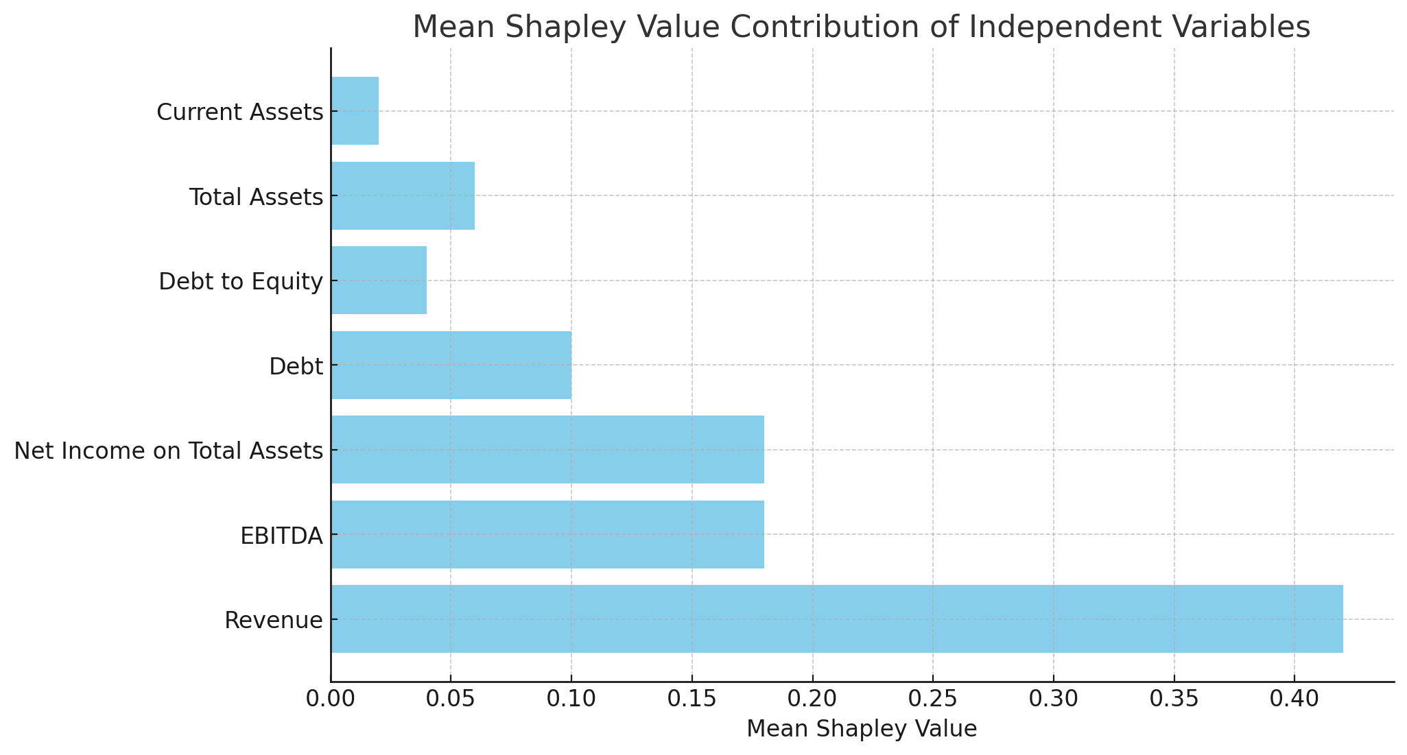
Applying the XGBoost model to balanced training data yielded an AUC of 0.91, indicating strong performance. However, to enhance interpretability, we calculated Shapley values, revealing Revenue as the most significant predictor of default probability. This insight is illustrated in Figure below.
Mean Shapley Value Contribution of Independent Variables
The bar chart below compares the Shapley value contributions of "Revenue" and "Leverage" for two defaulted and two non-defaulted companies, showcasing the influence of these variable on the predicted outcomes for individual enterprises.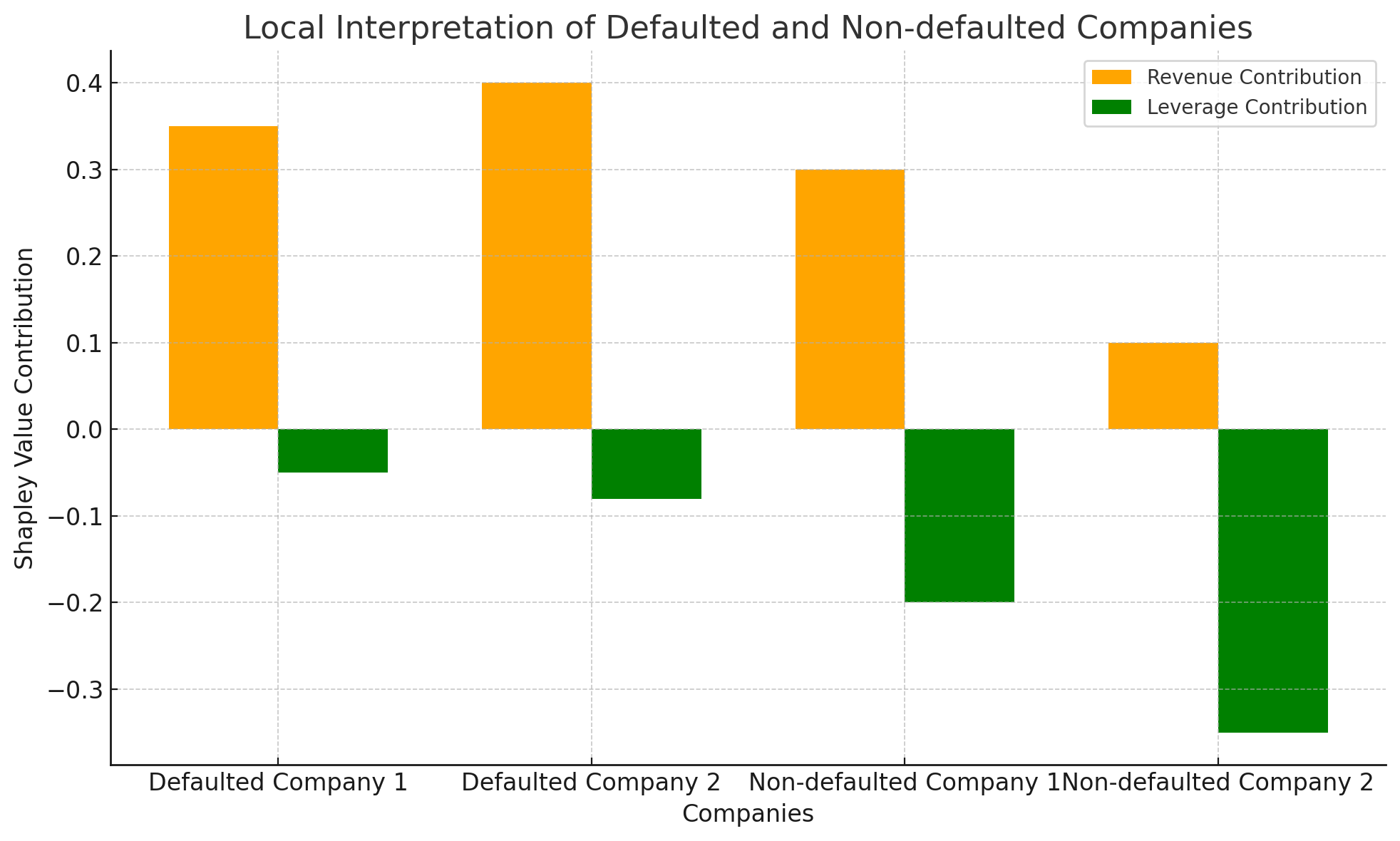
| Variable | Mean Shapley Value |
|---|---|
| Revenue | 0.42 |
| EBITDA | 0.18 |
| Net Income on Total Assets | 0.18 |
| Debt | 0.10 |
| Debt to Equity | 0.04 |
| Total Assets | 0.06 |
| Current Assets | 0.02 |
Local interpretations using Shapley values for individual enterprises highlighted that insufficient turnover was the primary cause of default for defaulted companies, while good turnover and low leverage explained the success of non-defaulted companies.
Conclusion
The complexity of ML models in enterprise analysis necessitates the use of explainable AI methods to make their predictions interpretable. By integrating Shapley values into our methodology, we provide a clear explanation of each financial indicator's contribution to the probability of default and expected return for each enterprise. This explainable model not only enhances understanding of company behavior but also supports informed investment decisions. Future research could explore other explainable AI methods and apply the proposed model to diverse case studies for broader validation.