Multi-Step Approach to Forecasting Financial Market Regimes Using Machine Learning and Factor Analysis

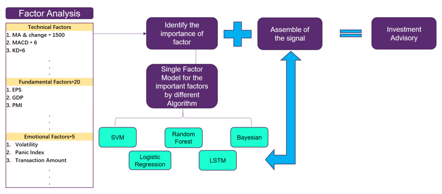
A versatile multi-step framework can exploit the power of machine learning and large datasets to forecast short-term financial market regimes. In this article, I will go over the steps to create a structured approach to use Machine Learning and Factor Analysis to Forecast Financial Market regimes sequentially.

Pre-Selecting the Most Informative Financial Predictors

The structured multi-step framework starts by pre-selecting the most informative financial predictors from a broad dataset. This initial step is crucial, as it helps identify the key variables that drive short-term financial market dynamics, while filtering out the noise and irrelevant information.

Techniques like sure independence screening can assess the individual predictive power of each variable, focusing the analysis on the most statistically significant ones. Alternatively, t-stat-based selection or Bayesian moving averaging can be used to identify the optimal subset of predictors.

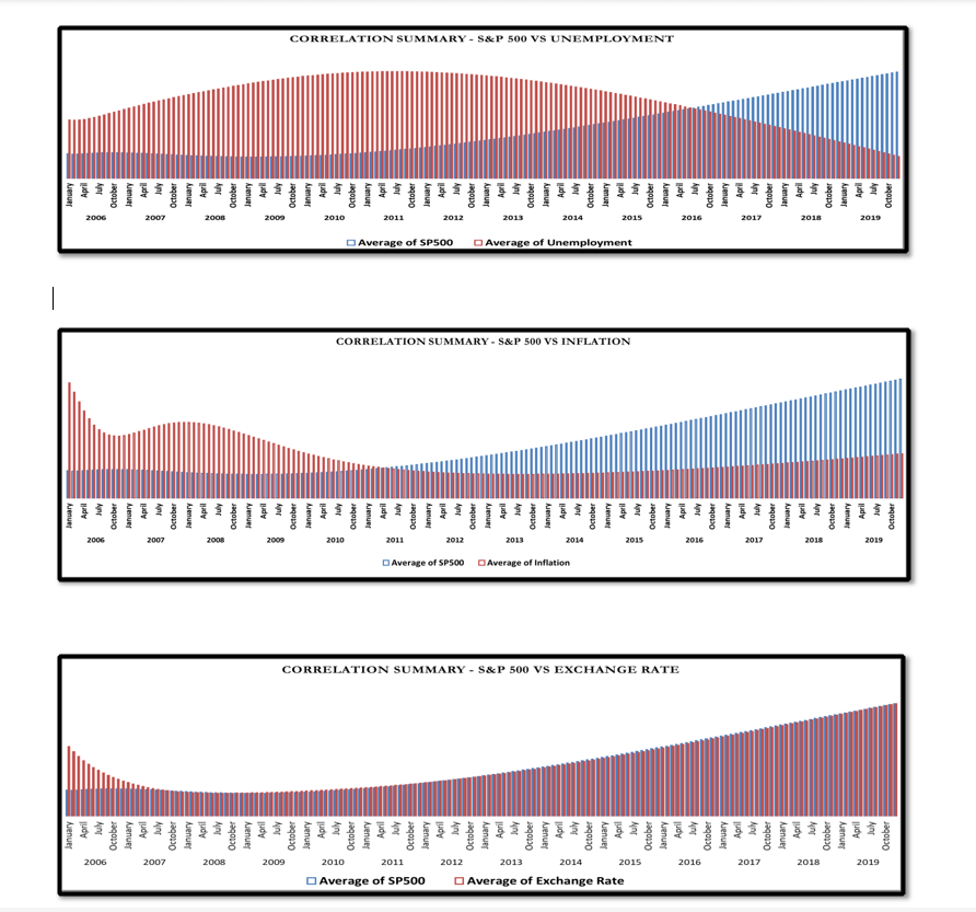
For example, in forecasting the S&P 500 index, the pre-selection stage may identify macroeconomic indicators like the unemployment rate, the yield curve slope, and consumer sentiment as the most relevant predictors, while filtering out less impactful variables like commodity prices or exchange rates.

Extracting Informative Factors from the Data

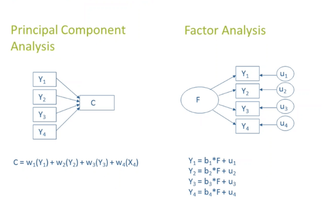
With the pre-selected financial variables in hand, the framework then extracts factors to summarize the information in a more parsimonious way. Principal Component Analysis (PCA) is a commonly used technique that identifies the orthogonal factors underlying the dataset. This data reduction step is crucial, as it helps eliminate idiosyncratic noise and collinearity issues that can plague financial forecasting models.

Continuing the S&P 500 example, PCA may distill the pre-selected macroeconomic variables into 3 or 4 key factors that capture the major sources of variation in the data, such as the business cycle, inflation expectations, and credit market conditions.

By structuring the forecasting process in this way - pre-selection, factor extraction, and non-linear modeling - the framework is able to deliver efficient and consistent predictions of short-term financial market regimes. This systematic approach has been shown to outperform traditional benchmarks, making it a valuable tool for fund managers, traders, and policymakers seeking to navigate the complexities of today's financial landscape.

This streamlined process is flexible and easy to implement, allowing it to adapt to diverse financial datasets and evolving market conditions. By strategically combining data reduction and advanced modeling, it can outperform benchmark approaches like the diffusion index method and dynamic factor models.

The Advantages of Factor-Based Financial Modeling

Incorporating factor analysis into the forecasting workflow offers several key benefits:

• Parsimony: Distilling a high-dimensional financial dataset into a few informative factors enhances model interpretability and performance.


• Noise Reduction: Factor extraction helps expel idiosyncratic noise, leading to more accurate financial predictions.


• Collinearity Mitigation: The orthogonal factors alleviate multicollinearity issues, further improving regression accuracy on financial variables.

Machine Learning Techniques for Financial Forecasting

Ones we obtained relevant features and extracted latent factors, we apply predictive modeling to leverage these extracted factors as explanatory variables in advanced machine learning regressions. Techniques like Markov switching can identify regime-dependent relationships, while quantile regression provides a more comprehensive view of the conditional financial distribution. Random forests and gradient boosting leverage the power of ensemble methods to achieve robust and accurate forecasts, especially during periods of financial market volatility. The structured forecasting framework leverages a diverse set of non-linear machine learning techniques, each tailored to specific financial modeling needs.

Markov Switching (MS) models are particularly well-suited for capturing regime-dependent dynamics in financial markets. By allowing model parameters to differ across unobserved states, MS can identify shifts in market conditions, such as transitions between bull and bear markets or changes in the volatility regime. For example, an MS model applied to the S&P 500 could distinguish between periods of low volatility and high volatility, providing valuable insights into the underlying financial risk factors.

Quantile Regression (QR) offers a more comprehensive view of the conditional financial distribution, going beyond just the mean. This is especially useful for risk management applications, as QR can estimate the growth-at-risk or the value-at-risk for a given financial asset or portfolio. In the context of the S&P 500, QR could estimate not only the expected index return, but also the potential downside risk at different confidence levels.

Random Forests (RF) are ensemble methods that leverage the power of many decision trees to achieve accurate and robust financial forecasts. By aggregating the predictions of multiple trees, RF can capture complex non-linear relationships in the data while mitigating the risk of overfitting. This makes RF a valuable tool for forecasting volatile financial variables, such as equity returns or credit spreads.

Finally, Gradient Boosting (GB) is another tree-based technique that iteratively builds an ensemble of weak learners to minimize the loss function. The linear gradient boosting (GB-L) variant uses linear regressions as the base learners, which can be particularly effective for financial time series that exhibit a stronger linear structure. GB-L has been successfully applied to forecasting macroeconomic variables like GDP growth and inflation, making it a promising approach for financial market predictions as well.

By harnessing this diverse array of non-linear machine learning methods, the structured forecasting framework can adapt to the unique characteristics and challenges of financial data, delivering accurate and reliable short-term predictions of market regimes.

Rigorous Real-Time Implementation for Financial Forecasting

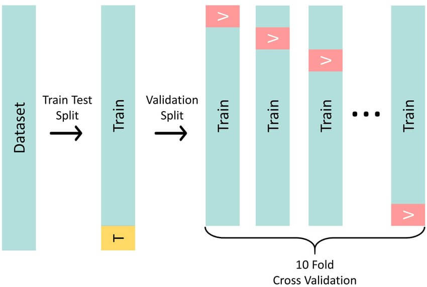
To ensure the structured forecasting framework remains robust and responsive in live financial settings, the model parameters and hyperparameters are recalibrated at each forecast date using a specialized cross-validation approach.

This real-time implementation is crucial, as financial markets are inherently dynamic and can undergo rapid changes in regime and structure. A model that performs well on historical data may quickly become obsolete if the underlying relationships shift, leading to deteriorating out-of-sample performance.

The cross-validation process works as follows: the in-sample period is split between a "test" sample, consisting of the last 12 monthly observations, and a "train" sample, made up of the remaining data. The model is then re-estimated on the train sample and its performance is evaluated on the test sample. This process is repeated iteratively, with the test sample sliding forward one month at a time, to simulate the real-time forecasting environment.

For example, when forecasting the S&P 500 index, the cross-validation may initially use data from January 2013 to January 2023 as the train sample, and January 2023 to January 2024 as the test sample. The next iteration would use February 2013 to February 2023 as the train sample, and February 2023 to February 2024 as the test sample, and so on.

By recalibrating the model parameters and hyperparameters (such as the number of trees in a random forest or the regularization strength in gradient boosting) at each step, the framework can adapt to changing market conditions and maintain its predictive accuracy. This dynamic adaptation is crucial, as financial markets can be heavily influenced by unexpected events, policy changes, and structural shifts that are difficult to capture with a static modeling approach.

Implementing this rigorous real-time setup ensures that the structured forecasting framework remains a reliable and responsive tool for predicting short-term financial market regimes, even as the underlying data and market dynamics evolve over time.